Abstract: Acceleration constrained hybrid dynamics calculations for a chain, based on Vereshchagin 1989. This class creates an instance of the hybrid dynamics solver. The solver analytically calculates the joint space constraint torques and acceleration in a chain when a constraint force(s) is applied to the chain's end-effector (task space / cartesian space). In the robotics literature, this algorithm is also known under the following names: Acceleration Constrained Hybrid Dynamics (ACHD) and Popov-Vereshchagin solver. More...
#include <chainhdsolver_vereshchagin.hpp>
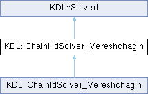
Public Member Functions | |
| ChainHdSolver_Vereshchagin (const Chain &chain, const Twist &root_acc, const unsigned int nc) | |
| ~ChainHdSolver_Vereshchagin () | |
| int | CartToJnt (const JntArray &q, const JntArray &q_dot, JntArray &q_dotdot, const Jacobian &alfa, const JntArray &beta, const Wrenches &f_ext, const JntArray &ff_torques, JntArray &constraint_torques) |
| virtual void | updateInternalDataStructures () |
| int | setDriverWeights (const Eigen::VectorXd &w_f_ext, const Eigen::VectorXd &w_ff_torques) |
| void | getTransformedLinkAcceleration (Twists &x_dotdot) |
| void | getTotalTorque (JntArray &total_tau) |
| void | getContraintForceMagnitude (Eigen::VectorXd &nu_) |
| Public Member Functions inherited from KDL::SolverI | |
| SolverI () | |
| Initialize latest error to E_NOERROR. | |
| virtual | ~SolverI () |
| virtual int | getError () const |
| Return the latest error. | |
| virtual const char * | strError (const int error) const |
Additional Inherited Members | |
| Public Types inherited from KDL::SolverI | |
| enum | { E_DEGRADED = +1 , E_NOERROR = 0 , E_NO_CONVERGE = -1 , E_UNDEFINED = -2 , E_NOT_UP_TO_DATE = -3 , E_SIZE_MISMATCH = -4 , E_MAX_ITERATIONS_EXCEEDED = -5 , E_OUT_OF_RANGE = -6 , E_NOT_IMPLEMENTED = -7 , E_SVD_FAILED = -8 } |
| Protected Attributes inherited from KDL::SolverI | |
| int | error |
| Latest error, initialized to E_NOERROR in constructor. | |
Detailed Description
Abstract: Acceleration constrained hybrid dynamics calculations for a chain, based on Vereshchagin 1989. This class creates an instance of the hybrid dynamics solver. The solver analytically calculates the joint space constraint torques and acceleration in a chain when a constraint force(s) is applied to the chain's end-effector (task space / cartesian space). In the robotics literature, this algorithm is also known under the following names: Acceleration Constrained Hybrid Dynamics (ACHD) and Popov-Vereshchagin solver.
INTRODUCTION
In 1970', researchers [1], [2] have developed a hybrid dynamics algorithm for evaluating robot behavior based on the input specification that is defined by the Cartesian acceleration constraints, feed-forward joint torques and external Cartesian wrenches. The solver is derived from a well-known principle of mechanics - Gauss' principle of least constraint [6] and provides an analytical (closed-form) solution to the hybrid dynamics problem with linear-time, O(n) complexity [3].
In general, the Gauss' principle states that the true motion (acceleration) of a system/body is defined by the minimum of a quadratic function that is subject to linear geometric motion constraints [7], [6]. The result of this Gauss function represents the acceleration energy of a body, which is defined by the product of its mass and the squared distance between its allowed (constrained) acceleration and its free (unconstrained) acceleration [10], [11]. In the case of originally derived Popov-Vereshchagin algorithm [1], geometric motion constraints are Cartesian acceleration constraints imposed on the robot's end-effector. This domain-specific solver minimizes the acceleration energy by performing computational (outward and inward) sweeps along the robot's kinematic chain [3]. Furthermore, by computing the minimum of Gauss function, the Popov-Vereshchagin solver resolves the kinematic redundancy of the robot, when a partial motion (task) specification is provided [2]. A necessary condition that enables this type of closed-form algorithm (an analytical solution to the above-described optimization problem) defines that the robot’s kinematic chain does not consist of closed loops, i.e. the robot’s kinematic chain must be constructed in a serial or tree structure [11]. However, it is always possible to cut these loops and introduce explicit constrains.
For evaluating robot dynamics, i.e. resolving its constrained motion, the Popov-Vereshchagin solver is performing three computational sweeps (recursions), along the kinematic chain [3]. More specifically, two sweeps in outward and one sweep in inward direction. In the case of robot dynamics algorithms, the outward sweep refers to a recursion that is covering a kinematic chain from proximal to distal segments, while the inward sweep is covering a kinematic chain from distal to proximal segments [5]. Additionally, after completing the recursion in the second sweep and before starting the recursion in the last sweep, the solver is computing magnitudes of constraint forces, i.e. the Langrage multiplier (noted as nu in the KDL's solver implementation and original solver's publication[2]). More specifically, this operation is performed when the algorithm reaches segment (link) **{0}**, namely the base segment. In this formulation of the solver, the gravity effects are taken into account by setting the base-link's acceleration equal to gravitational acceleration [3].
For more detailed description of the algorithm and its representation, the reader can refer to [3], [5], [11].
INTERFACES
Solver's Input
For computing solutions to the constrained hybrid dynamics problem, this original derivation of the Popov-Vereshchagin solver [3] takes into account the following inputs:
- Robot's model defined by: kinematic parameters of the chain, segments' mass and rigid-body inertia, and effective inertia of each joint rotor -> chain parameter in solver's constructor
- Root acceleration of the robot's base segment (usually gravitational) -> root_acc parameter in solver's constructor
- Current joint configuration (angles) -> q parameter in the CartToJnt function
- Current joint velocities -> q_dot parameter in the CartToJnt function
- Motion drivers:
- - Cartesian Acceleration Constraints imposed on the end-effector segment -> alpha and beta parameters in the CartToJnt function
- - Cartesian External Wrench acting on each segment -> f_ext parameter in the CartToJnt function
- - Feed-Forward Torque acting on each joint -> ff_torques parameter in the CartToJnt function
The following outlines the above-listed task interfaces in more detail.
Cartesian Acceleration Constraints: alpha & beta
This first type of motion driver can be used for specifying physical constraints such as contacts with environment [3], or artificial (i.e. task-imposed) constraints defined by the operational space task definition for the end-effector (tool-tip) segment. Note: the Vereshchagin solver expects that the input Cartesian Acceleration Constraints, i.e. unit constraint forces in alpha parameters, are expressed w.r.t. robot's base frame. However, the acceleration energy setpoints, i.e. beta parameters, are expressed w.r.t. above-defined unit constraint forces. More specifically, each DOF (element) in beta parameter corresponds to its respective DOF (column) of the unit constraint force matrix (alpha) [11].
To use this interface, a user should define i) the active constraint directions via alpha parameter, which is a 6 x m matrix of spatial unit constraint forces, and ii) acceleration energy setpoints via beta, which is a m x 1 vector. Here, the number of constraints m, or in another words number of spatial unit constraint forces is not required to always be equal to 6, which means that a human programmer can leave some of the degrees of freedom unspecified [2] for this motion driver, and still produce valid joint control commands [5]. For example, if we want to constrain the motion of the end-effector segment in only one direction, namely linear x-direction, we can define the constraint as [3]:
alpha =
| 1 |
| 0 |
| 0 |
| 0 |
| 0 |
| 0 |
beta = | 0 |
Note that here, the first three rows of matrix alpha represent linear elements and the last three rows represent angular elements, of the spatial unit force defined in Plücker coordinates [4]. By giving zero value to acceleration energy setpoint (beta), we are defining that the end-effector is not allowed to have linear acceleration in x direction. Or in other words, we are restricting the robot from producing any acceleration energy in that specified direction.
Another example includes the specification of constraints in 5 DOFs. We can constrain the motion of robot's end-effector such that it is only allowed to freely move in the linear z-direction, without performing linear motions in x and y and angular motions in x, y and z directions:
alpha =
| 1 | 0 | 0 | 0 | 0 |
| 0 | 1 | 0 | 0 | 0 |
| 0 | 0 | 0 | 0 | 0 |
| 0 | 0 | 1 | 0 | 0 |
| 0 | 0 | 0 | 1 | 0 |
| 0 | 0 | 0 | 0 | 1 |
beta =
| 0 |
| 0 |
| 0 |
| 0 |
| 0 |
For both above-described task examples, the Acceleration Constrained Hybrid Dynamics (ACHD) solver will compute valid control (constraint) joint torques, even though some of the Cartesian DOFs are left unspecified (e.g. in the case of the second example that would be end-effector's z-direction). More specifically: Underconstrained motion specifications are naturally resolved using Gauss' principle of least constraint [5]. This means that in those directions in which the robot is not constrained by the task definition, its motions will be controlled by the nature. For instance, in the second example, natural resolution of the robot motion would define that the end-effector "**falls**" in the linear z direction due to effects of gravity, with the assumption that gravity forces are acting along $z$-direction.
Moreover, the motion specification in the second example is equivalent to:
alpha =
| 1 | 0 | 0 | 0 | 0 | 0 |
| 0 | 1 | 0 | 0 | 0 | 0 |
| 0 | 0 | 0 | 0 | 0 | 0 |
| 0 | 0 | 0 | 1 | 0 | 0 |
| 0 | 0 | 0 | 0 | 1 | 0 |
| 0 | 0 | 0 | 0 | 0 | 1 |
(note that elements in the third column are all zeros, meaning z-linear constraint is deactivated)
beta =
| 0 |
| 0 |
| 0 |
| 0 |
| 0 |
| 0 |
The last example involves the full specification of the desired end-effector motion (in this case, not necessarily zero accelerations), i.e. specification of constraints in all 6 DOFs:
alpha =
| 1 | 0 | 0 | 0 | 0 | 0 |
| 0 | 1 | 0 | 0 | 0 | 0 |
| 0 | 0 | 1 | 0 | 0 | 0 |
| 0 | 0 | 0 | 1 | 0 | 0 |
| 0 | 0 | 0 | 0 | 1 | 0 |
| 0 | 0 | 0 | 0 | 0 | 1 |
beta = alpha^T * X_dotdot_N
Here, N stands for the index of the last robot's segment, end-effector (tool-tip). The reader should note that we can directly assign values (magnitudes) of the desired (task-defined) spatial acceleration 6 x 1 vector X_dotdot_N to the 6 x 1 vector of acceleration energy (beta) [3]. Even though physical dimensions (units) of these two vectors are not the same, the property of matrix alpha (it contains unit vectors), permits that we can assign values of desired accelerations to acceleration energy setpoints, in respective directions. Namely, each column of matrix alpha has the value of 1 in the respective direction in which constraint force works, thus it follows that the value of acceleration energy setpoint is the same as the value of Cartesian acceleration, in the respective direction.
A note on gravity: beta and the reported accelerations are true accelerations
This solver takes gravity into account by setting the root_acc parameter (passed to the constructor) to the negative of the gravitational acceleration [4], so internally every Cartesian acceleration is offset by root_acc. That offset never reaches the interface: beta is the acceleration energy of the true base-frame acceleration, beta = alpha^T * X_dotdot_desired, and getTransformedLinkAcceleration and the other acceleration getters return true base-frame accelerations. In particular, beta = 0 in a constrained direction holds the end-effector's acceleration at zero there; at rest it stays at rest, carried by the constraint torque. Internally the solver adds alpha^T * root_acc to beta before the balance of Eq. (3.37) in [3] and subtracts root_acc from the accelerations it reports.
External Forces: f_ext
This type of driver can be used for specifying physical (but not artificial, i.e. not task-introduced) Cartesian wrenches acting on each of the robot's segments [11]. Examples for a physical force on a segment can be: i) a known weight at the robot's gripper, for instance, a grasped cup or ii) a force from a human pushing the robot [5]. Note that the implementation of Vereshchagin solver in KDL expects the provided f_ext is expressed w.r.t. robot's base frame, which is in contrast to the case of KDL's RNE solver.
Feed-Forward Joint Torques: ff_torque
This type of motion driver can be used for specifying physical (but not artificial, i.e. not task-introduced) joint torques, for example, spring and/or damper-based torques (e.g. friction effects) in robot's joints [11].
Additional examples on using these input interfaces can be found in "../tests/solvertest.cpp":
- VereshchaginTest() function - an example on how to use all interfaces of this solver for computing the solution to the Hybrid Dynamics (HD) problem.
- FdAndVereshchaginSolversConsistencyTest() function - an example on how to only use this solver for computing the solution to the Featherstone's (i.e. Articulated Body Algorithm (ABA)) version of the Forward Dynamics (FD) problem.
Solver's Output
This recursive dynamics solver is computing several quantities that represent solutions to both, inverse and forward dynamics problems, or in other words solutions to the constrained hybrid dynamics problem. More specifically, the output interface of the original Popov-Vereshchagin algorithm consists of [3], [5]:
- Magnitudes of constraint forces that act on the end-effector, denoted by the Lagrange multiplier nu in the solver's implementation and original solver's publication[2].
- Joint constraint torques required for achieving the desired (acceleration-constraints-defined) behavior of the robot: constraint_torque. These torques represent control commands that should be sent to robot's joint drivers.
- Argument that defines the solution to the originally formulated optimization problem in Gauss' principle. In other words, the joint accelerations q_dotdot resulting from the total torque acting on each joint (total_torque), i.e. from the aforementioned constraint torques and all natural and external forces acting on the system.
- The resulting and complete spatial accelerations of each segment in the kinematic chain: X_dotdot
Furthermore, if necessary, a complete spatial vector of imposed constraint forces can be computed [3], from the following relation: alpha * nu.
The reader should note that this constraint_torque is the necessary control command that a user is supposed to send to robot's joints, to achieve the motion that is computed (resolved) by the Popov-Vereshchagin solver. More specifically, here constraint_torque represent solution to the Inverse Dynamics (ID) problem. Nevertheless, the reason why a user is not supposed to use the total_torque values as the control commands for robot's joints, is the fact that the torque contributions that represent the difference between total_torque and constraint_torque already exist (act) on robot joints. More specifically, these additional (residual) contributions are produced on the joints by the already existing natural forces that act on the system [11].
On the other side, joint accelerations, namely q_dotdot provide solution to the Forward Dynamics (FD) problem and these quantities can be used for both control (integrate to joint positions/velocities) and simulation purposes [11].
PRACTICAL INSIGHTS/CONSIDERATIONS
The Popov-Vereshchagin hybrid dynamics solver enables a user to achieve many types of operational space tasks [11]. In other words, various controllers can be implemented around the aforementioned interfaces of the algorithm. Examples can be controllers for hybrid force/position control, impedance control, etc. However, there are some practical insights about this algorithm that need to taken into account.
Prioritizations between motion drivers (interfaces)
The original derivation of this solver, which is considered in this library, prioritizes Cartesian acceleration constrains (specified for the end-effector segment) over other two motion drivers (Cartesian external wrenches and feedforward joint torques) [11]. In practice, this means the following:
- If the external wrenches and/or feedforward joint torques contribute positively (i.e. assist) in producing Cartesian accelerations (specified via acceleration constraint interface), the Vereshchagin solver will take advantage of these forces to compute (acceleration-) energy optimal motions.
- On the other hand, if the aforementioned external wrenches and/or feedforward joint torques contribute negatively (i.e. interfere) the Cartesian accelerations, the Vereshchagin solver will compensate all of those forces to correctly produce constrained accelerations of the end-effector. More specifically, additional torque commands will be computed under constrained joint torques (ctrl_torques in this implementation), to overcome those "disturbances".
Nevertheless, the above-described prioritization can be changed (see [3] & [5] for more details), via setDriverWeights.
Changing the prioritization: setDriverWeights
The setDriverWeights method accepts two nc x 1 weight vectors, one per constraint direction (the columns of alpha): one for the external wrenches (f_ext) and one for the feed-forward joint torques (ff_torques). Following Eq. (3.42) of [3], b_control = w_posture * b_posture + w_ee * b_ee, each weight is the share of the acceleration energy that driver generates at the end-effector which is added to the constraint target, i.e. the share the constraint leaves uncompensated:
- w = 0 (the default) – the constraint fully compensates that driver in that direction, reproducing the classic Popov-Vereshchagin prioritization described above.
- w = 1 – the driver passes through: the end-effector accelerates by the constrained setpoint plus the acceleration that driver alone would produce. The joint accelerations then change by exactly M^-1 * J^T * f_ext (or M^-1 * ff_torques) with respect to the same solve without the driver.
- 0 < w < 1 – a linear blend of the two.
Eq. (3.42)'s w_ee (the weight on the setpoint itself) is not a separate parameter: scale beta.
Because the weights are vectors rather than scalars, this can be applied per constraint direction, e.g. compliant along a contact normal while remaining stiff in the other constrained directions.
Note what f_ext means under a non-zero weight. The solver treats f_ext as a force acting on the segment. With w = 0 that is a disturbance the constraint rejects, e.g. a measured contact force. With w = 1 the arm's motion (and, through inverse dynamics, its joint torque) carries the full J^T * f_ext, which is what a controller uses to make the arm exert a modelled wrench on the environment. Sensed and commanded wrenches enter through the same input; the weight decides which one it is.
Using the algorithm for solving forward dynamics (FD) problem
The reader should note that the Popov-Vereshchagin solver represents an extension to the well-known forward-dynamics Articulated Body Algorithm (ABA) developed by Featherstone and described in [4] (moreover, Featherstone mentioned Vereshchagin solver in his book [4], page 117). This means that the Popov-Vereshchagin solver can also be purely used as this Articulated Body Algorithm forward-dynamics algorithm. In that case, it is necessary for the user to deactivate all Cartesian acceleration constraints (it is sufficient to set all elements in alpha matrix to zero) and proceed using other two interfaces as in the case of standard FD solver. More specifically, use f_ext input to define physical external wrenches acting on the robot's body (should be expressed w.r.t. robot's base frame) and ff_torque input to define command torques acting in robot's joints. The resulting robot's motion can be taken from q_dotdot and X_dotdot solver's outputs.
Nevertheless, the Popov-Vereshchagin solver can also be used for solving more advanced forward dynamics problems, than those solved by ABA [4]. More specifically, if this solver is used in a certain simulation environment for the use-case of simulating robot behaviors, all three interfaces can be exploited for defining a more descriptive robot's state. Here, a user can exploit the Cartesian acceleration constraint interface to specify different constraints imposed on the end-effector, along with other interfaces, and simulate what would be the robot's behavior due to these constraints and environmental impacts. Here, the resulting robot's motion can, as well, be taken from q_dotdot and X_dotdot solver's outputs. For example, MuJoCo framework (see MuJoCo's documentation) also uses Gauss' principle of least constraint to simulate constraint forces in certain situations, however, there, final derivation of this principle in the software is different. However, in the case of this more advanced forward dynamics computations, the user needs to be aware of prioritizations between input interfaces (mentioned in "Prioritizations" section above) and internal policies on handling singularities (mentioned in "Singularities and matrix inversions" section below).
Singularities and matrix inversions
To find the minimal-energy solution to the Inverse Dynamics (ID) problem, i.e. find the Langrage multiplier nu, the solver needs to compute the inverse of a so-called "acceleration constraint coupling matrix"[3] in the balance equation before starting the third sweep. However, the robot's configuration has a direct impact on this matrix and its inversion. Namely, if the robot is in a singular configuration for the task specified via acceleration constraints, this matrix will become rank-deficient. This means that it is not possible to find a feasible solution for that particular end-effector's DOF that is (or DOFs that are) lost due to the singular configuration. In other words, it is not possible to find constraint torques that will satisfy imposed acceleration constraints in that DOF/DOFs. Nevertheless, in this situation, it is still possible to find the (energy-optimal) solution for other "non-singular" DOFs. For that reason, in KDL's implementation of the solver, matrix inverse is found by using the SVD technique to construct a pseudo inverse. Additionally, in this implementation, a control policy is introduced via the truncated-SVD method to deactivate, i.e. more specifically ignore, acceleration constraints for the DOFs that are lost due to robot's singular configuration. Of course, this is a choice (control policy), i.e. only one option for solving the singularity problem and producing safe joint commands. It is left for the user to explore other control policies (options) for this particular problem if of course, the user is not satisfied with the current control policy.
Supported robot models
Segments with a Joint::Fixed joint are supported: such a segment carries its pose and inertia but no degree of freedom, so a chain may have fewer joints than segments. All joint-space inputs and outputs (q, q_dot, q_dotdot, ff_torques, constraint_torques) are sized by the number of joints, while f_ext has one entry per segment. This implementation can only compute dynamics for serial type of chains, i.e. currently, tree robot structures are not supported in this solver. Nevertheless, the original solver's derivation has been extended in [3] to account for multiple motion constraints imposed on a tree robot structure. This extension does not only account for acceleration constraints imposed on multiple end-effectors but also for acceleration constraints imposed on more proximal segments. However, the above-mentioned extensions are currently not implemented in this version of KDL.
REFERENCES
[1] E. P. Popov, A. F. Vereshchagin, and S. L. Zenkevich, "Manipulyatsionnye roboty: Dinamika i algoritmy", Nauka, Moscow, 1978.
[2] A. F. Vereshchagin, “Modelling and control of motion of manipulation robots”, Soviet Journal of Computer and Systems Sciences, vol. 27, pp. 29–38, 1989.
[3] A. Shakhimardanov, “Composable robot motion stack: Implementing constrained hybrid dynamics using semantic models of kinematic chains”, PhD thesis, KU Leuven, 2015.
[4] R. Featherstone, Rigid body dynamics algorithms. Springer, 2008.
[5] S. Schneider and H. Bruyninckx, “Exploiting linearity in dynamics solvers for the design of composable robotic manipulation architectures”, in IEEE/RSJ International Conference on Intelligent Robots and Systems (IROS), 2019.
[6] H. Bruyninckx and O. Khatib, "Gauss’ principle and the dynamics of redundant and constrained manipulators", in IEEE International Conference on Robotics and Automation, 2000.
[7] C. F. Gauß, "Über ein neues allgemeines Grundgesetz der Mechanik.", Journal für die reine und angewandte Mathematik, vol. 4, pp. 232–235, 1829.
[8] A. F. Vereshchagin, “Computer simulation of the dynamics of complicated mechanisms of robot-manipulators”, Engineering Cybernetics, 12(6), pp. 65–70, 1974.
[9] E. P. Popov, "Control of robots-manipulators", Engineering Cybernetics, 1974.
[10] E. Ramm, “Principles of least action and of least constraint”, GAMM-Mitteilungen, vol. 34, pp. 164–182, 2011.
[11] D. Vukcevic, "Lazy Robot Control by Relaxation of Motion and Force Constraints." Technical Report/Hochschule Bonn-Rhein-Sieg University of Applied Sciences, Department of Computer Science, 2020.
Constructor & Destructor Documentation
◆ ChainHdSolver_Vereshchagin()
| KDL::ChainHdSolver_Vereshchagin::ChainHdSolver_Vereshchagin | ( | const Chain & | chain, |
| const Twist & | root_acc, | ||
| const unsigned int | nc ) |
Constructor for the solver, it will allocate all the necessary memory
- Parameters
-
chain The kinematic chain to calculate the hybrid dynamics for. An internal copy will be made. root_acc The acceleration twist of the root segment to use during the calculation (usually contains gravity). Note: This solver takes gravity acceleration with opposite sign comparead to the KDL's FD and RNE solvers nc Number of constraints imposed on the robot's end-effector (maximum is 6).
◆ ~ChainHdSolver_Vereshchagin()
|
inline |
Member Function Documentation
◆ CartToJnt()
| int KDL::ChainHdSolver_Vereshchagin::CartToJnt | ( | const JntArray & | q, |
| const JntArray & | q_dot, | ||
| JntArray & | q_dotdot, | ||
| const Jacobian & | alfa, | ||
| const JntArray & | beta, | ||
| const Wrenches & | f_ext, | ||
| const JntArray & | ff_torques, | ||
| JntArray & | constraint_torques ) |
This method calculates joint space constraint torques and accelerations. It returns 0 when it succeeds, otherwise -1 or -2 for nonmatching matrix and array sizes. Input parameters:
- Parameters
-
q The current joint positions q_dot The current joint velocities alpha The active constraint directions (unit constraint forces expressed w.r.t. robot's base frame) beta The acceleration energy setpoints (expressed w.r.t. above-defined unit constraint forces) f_ext The external forces (no gravity, it is given in root acceleration) on the segments ff_torques The feed-forward joint space torques
Output parameters:
- Parameters
-
q_dotdot The resulting joint accelerations constraint_torques The resulting joint constraint torques (what each joint feels due to the constraint forces acting on the end-effector)
- Returns
- error/success code
◆ getContraintForceMagnitude()
| void KDL::ChainHdSolver_Vereshchagin::getContraintForceMagnitude | ( | Eigen::VectorXd & | nu_ | ) |
◆ getTotalTorque()
| void KDL::ChainHdSolver_Vereshchagin::getTotalTorque | ( | JntArray & | total_tau | ) |
◆ getTransformedLinkAcceleration()
| void KDL::ChainHdSolver_Vereshchagin::getTransformedLinkAcceleration | ( | Twists & | x_dotdot | ) |
◆ setDriverWeights()
| int KDL::ChainHdSolver_Vereshchagin::setDriverWeights | ( | const Eigen::VectorXd & | w_f_ext, |
| const Eigen::VectorXd & | w_ff_torques ) |
Set the per-driver pass-through weights used when solving for the constraint force magnitudes. Each weight is an nc-vector, one entry per column of alpha.
A weight of 0.0 (the default) means the acceleration constraint fully compensates that driver, i.e. the constraint is satisfied exactly regardless of the driver – this is the classic Popov-Vereshchagin prioritisation. A weight of 1.0 means the driver passes through: the constrained segment accelerates by the setpoint plus what that driver alone would produce. Values in between blend the two, as in Eq. (3.42) of [3], whose w_posture this is.
- Parameters
-
w_f_ext pass-through share per constraint direction for the external wrenches w_ff_torques pass-through share per constraint direction for the feed-forward joint torques
- Returns
- E_NOERROR on success, E_SIZE_MISMATCH if either vector is not of size nc
◆ updateInternalDataStructures()
|
virtual |
Update the internal data structures. This is required if the number of segments or number of joints of a chain/tree have changed. This provides a single point of contact for solver memory allocations.
Implements KDL::SolverI.
The documentation for this class was generated from the following file:
- build/orocos_kdl_install/include/kdl/chainhdsolver_vereshchagin.hpp
Generated by
 1.16.1